Basics
SeismicMesh supports the generation of both 2D and 3D meshes in either serial or parallel from seismic velocity models.
Here I show how to build meshes from sizing functions created with the software and explain what the sizng options mean. The API for serial/parallel and 2D/3D is identical.
Assuming you’ve coded a short Python script to call SeismicMesh (similar to what is shown in the examples), you simply call the script with python for serial execution:
python your_script.py
Distributed memory parallelism can be used by first writing an extra import statement for mpi4py (import mpi4py) near your other imports. Following this write the following line near the top of your script before you call the SeismicMesh API):
comm = MPI.COMM_WORLD
Note
This line has no effect on serial execution and its fine to leave it in if you intend to only use serial execution.
Parallel execution takes place by typing by:
mpiexec -n N python your_script.py
where N is the number of cores (e.g., 2,3,4 etc.)
Warning
Oversubscribing the mesh generation problem to too many cores will surely lead to problems and slow downs. In general, keeping the minimum number of vertices per rank to between 20-50k/rank results in optimal performance.
Example data
Note
Users should create a directory called velocity_models and place their seismic velocity models there.
A 2D model (BP2004):
wget http://s3.amazonaws.com/open.source.geoscience/open_data/bpvelanal2004/vel_z6.25m_x12.5m_exact.segy.gz
A 3D model (EAGE Salt):
https://s3.amazonaws.com/open.source.geoscience/open_data/seg_eage_models_cd/Salt_Model_3D.tar.gz
File I/O and visualization of meshes
Meshes can be written to disk in a variety of formats using the Python package meshio (https://pypi.org/project/meshio/).
Warning
Note that SeismicMesh sizing function makes the assumption that the first dimension is z and the second is x while the third is y. This is done in this way since 2D seismological simulations take place in the z-x plane and 3D in the z-x-y plane. As a result, the meshes when loaded into visualization software will appear rotated 90 degrees. For visualization, we can output in the vtk format using MeshIO (as shown in the examples) and then load the vtk file into ParaView.
Some things to know
This seismic velocity model is passed to the get_sizing_function_from_segy along with the domain extents
from SeismicMesh import get_sizing_function_from_segy

# Construct a mesh sizing function from a seismic velocity model
ef = get_sizing_function_from_segy(fname, bbox, other-args-go-here,...)
- The user specifies the filename fname of the seismic velocity model (e.g., either SEG-y or binary)
- The user specifies the domain extents of the velocity model as a tuple of coordinates in meters representing the corners of the domain:
- In 3D:
Geometry
SeismicMesh can mesh any domain defined by a signed distance function. However, we provide some basic domain shapes: a rectangle, a cube, or a disk.
For example:
from SeismicMesh import Rectangle, Cube, Disk

rectangle = Rectangle(bbox)
cube = Cube(bbox)
disk = Disk(x0=[0,0],r=1) # center of (0,0) with a radius of 1.0
Note
A good reference for various signed distance functions can be found at: https://www.iquilezles.org/www/articles/distfunctions/distfunctions.htm
Mesh size function
The notion of an adequate mesh size is determined by a combination of the physics of acoustic/elastic wave propagation, the desired numerical accuracy of the solution (e.g., spatial polynomial order, timestepping method, etc.), and allowable computational cost of the model amongst other things. In the following sub-sections, each available mesh sizing strategy is briefly described and pseudo code is provided.
Note
The final mesh size map is taken as the minimum of all supplied sizing functions.
Note
The mesh size map dictates the triangular edge lengths in the final mesh (assuming these triangles will be equilateral).
Wavelength-to-gridscale
The highest frequency of the source wavelet \(f_{max}\) and the smallest value of the velocity model \(v_{min}\) define the shortest scale length of the problem since the shortest spatial wavelength \(\lambda_{min}\) is equal to the \(\frac{v_{min}}{f_{max}}\). For marine domains, \(v_{min}\) is approximately 1,484 m/s, which is the speed of sound in seawater, thus the finest mesh resolution is near the water layer.
The user is able to specify the number of vertices per wavelength \(\alpha_{wl}\) the peak source frequency \(f_{max}\). This sizing heuristic also can be used to take into account varying polynomial orders for finite elements. For instance if using quadratic P=2 elements, \(\alpha_{wl}\) can be safely be set to 5 to avoid excessive dispersion and dissipation otherwise that would occur with P=1 elements:
# Construct mesh sizing object from velocity model
ef = get_sizing_function_from_segy(fname, bbox,
    wl=3, # :math:`\alpha_{wl}` number of grid points per wavelength
    freq=2, # maximum source frequency for which the wavelength is calculated
)
Resolving seismic velocity gradients
Seismic domains are known for sharp gradients in material properties, such as seismic velocity. These sharp gradients lead to reflections and refractions in propagated waves, which are critical for successful imaging. Thus, finer mesh resolution can be deployed inversely proportional to the local standard deviation of P-wave velocity. The local standard deviation of seismic P-wave velocity is calculated in a sliding window around each point on the velocity model. The user chooses the mapping relationship between the local standard deviation of the seismic velocity model and the values of the corresponding mesh size nearby it. This parameter is referred to as the \(grad\) and is specified in meters. For instance a \(grad\) of 50 would imply that the largest gradient in seismic P-wave velocity is mapped to a minimum resolution of 50-m.:
ef = get_sizing_function_from_segy(fname, bbox,
    grad=50, # the desired mesh size in meters near the sharpest gradient in the domain
)
Courant-Friedrichs-Lewey (CFL) condition
Almost all numerical wave propagators utilize explicit time-stepping methods in the seismic domain. The major advantage for these explicit methods is computational speed. However, it is well-known that all explicit or semi-explicit methods require that the Courant number be bounded above by the Courant-Friedrichs-Lewey (CFL) condition. Ignoring this condition will lead to a numerically unstable simulation. Thus, we must ensure that the Courant number is indeed bounded for the overall mesh size function.
After sizing functions have been activated, a conservative maximum Courant number is enforced.
For the linear acoustic wave equation assuming isotropic mesh resolution, the CFL condition is commonly described by
where \(h\) is the diameter of the circumball that inscribes the element either calculated from \(f(h)\) or from the actual mesh cells, \(dim\) is the spatial dimension of the problem (2 or 3), \(\Delta t\) is the intended simulation time step in seconds and \(v_p\) is the local seismic P-wave velocity. The above equation can be rearranged to find the minimum mesh size possible for a given \(v_p\) and \(\Delta t\), based on some user-defined value of \(Cr \leq 1\). If there are any violations of the CFL, they can bed edited before building the mesh so to satisfy that the maximum \(Cr\) is less than some conservative threshold. We normally apply \(Cr = 0.5\), which provides a solid buffer but this can but this can be controlled by the user like the following:
ef = get_sizing_function_from_segy(fname, bbox,
    cr=0.5, # maximum bounded Courant number to be bounded in the mesh sizing function
    dt=0.001, # for the given :math:`\Delta t` of 0.001 seconds
    ...
)
Further, the space order of the method (\(p\)) can also be incorporated into the above formula to consider the higher spatial order that the simulation will use:
ef = get_sizing_function_from_segy(fname, bbox,
    cr=0.5, # maximum bounded Courant number :math:`Cr_{max}` in the mesh
    dt=0.001, # for the given :math:`\Delta t` of 0.001 seconds
    space_order = 2, # assume quadratic elements :math:`P=2`
    ...
)
The above code implies that the mesh will be used in a simulation with \(P=2\) quadratic elements, and thus will ensure the \(Cr_{max}\) is divided by \(\frac{1}{space\_order}\)
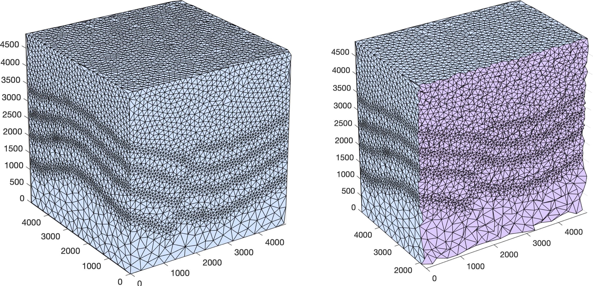
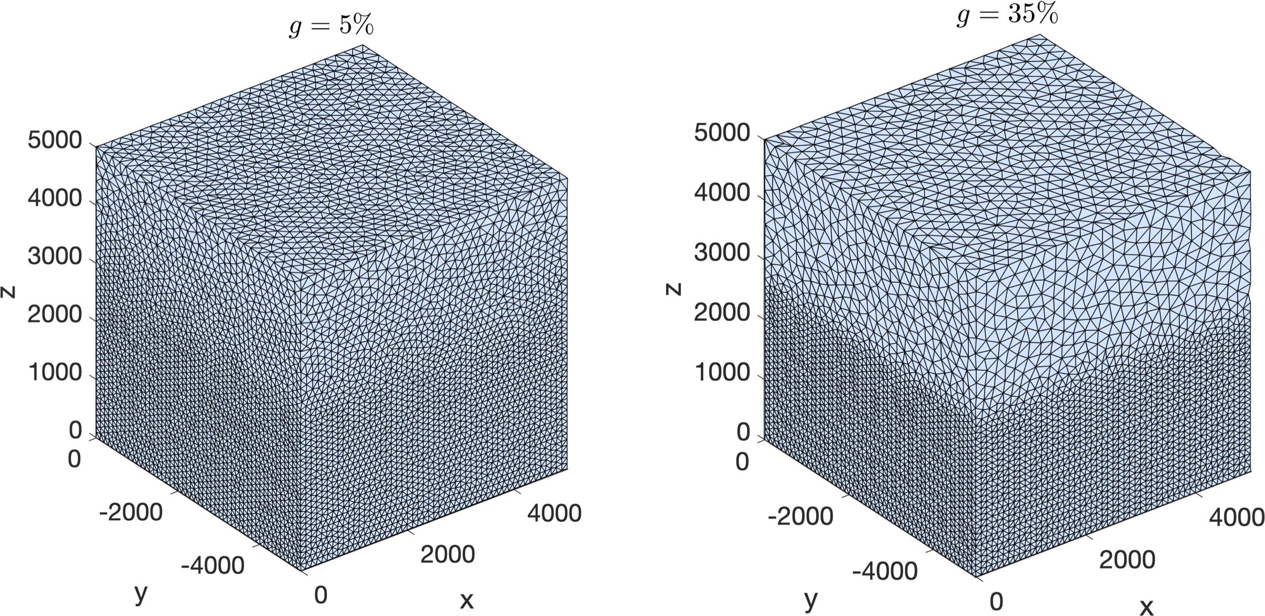
Mesh size gradation
In regions where there are sharp material contrasts, the variation in element size can become substantially large, especially using the aforementioned sizing strategies such as the wavelength-to-gridscale. Attempting to construct a mesh with such large spatial variations in mesh sizes would result in low-geometric quality elements that compromise the numerical stability of a model.
Thus, the final stage of the development of a mesh size function \(h(x)\) involves ensuring a size smoothness limit, \(g\) such that for any two points \(x_i\), \(x_j\), the local increase in size is bounded such as:
\(h(\boldsymbol{x_j}) \leq h(\boldsymbol{x_i}) + \alpha_g||\boldsymbol{x_i}-\boldsymbol{x_j}||\)
A smoothness criteria is necessary to produce a mesh that can simulate physical processes with a practical time step as sharp gradients in mesh resolution typically lead to highly skewed angles that result in poor numerical performance.
We adopt the method to smooth the mesh size function originally proposed by [grading]. A smoother sizing function is congruent with a higher overall element quality but with more triangles in the mesh. Generally, setting \(0.2 \leq \alpha_g \leq 0.3\) produces good results:
ef = get_sizing_function_from_segy(fname, bbox,
    ...
    grade=0.15, # :math:`g` cell-to-cell size rate growth bound
    ...
)
Domain padding
Note
It is assumed that the top side of the domain represents the free-surface thus no domain padding applied there.
In seismology applications, the goal is often to model the propagation of an elastic or acoustic wave through an infinite domain. However, this is obviously not possible so the domain is approximated by a finite region of space. This can lead to undesirable artificial reflections off the sides of the domain however. A common approach to avoid these artificial reflections is to pad the domain and enforce absorbing boundary conditions in this extension. In terms of meshing to take this under consideration, the user has the option to specify a domain extension of variable width on all three sides of the domain like so:
ef = get_sizing_function_from_segy(fname, bbox,
    domain_pad=250, # domain will be pad by 250-m on all three sides of the domain
    ...
)
In this domain pad, mesh resolution can be adapted according to following three different styles.
Linear- pads the seismic velocities on the edges of the domain linearly increasing into the domain pad.Constant- places a constant velocity of the users selection in the domain pad.Edge- pads the seismic velocity about the domain boundary so that velocity profile is identical to its edge values.
An example of the edge style is below:
ef = get_sizing_function_from_segy(fname, bbox,
    domain_pad=250, # domain will be extended by 250-m on all three sides
    padstyle="edge", # velocity will be extend from values at the edges of the domain
    ...
)
Note
In our experience, the edge option works the best at reducing reflections with absorbing boundary conditions.
Mesh generation
After building your signed distance function and sizing function, call the generate_mesh function to generate the mesh:
points, cells = generate_mesh(domain=rectangle, edge_length=ef, h0=hmin)
Note
ef is a sizing function created using get_sizing_function_from_segy
You can change how many iterations are performed by altering the kwarg max_iter:
points, cells = generate_mesh(domain=rectangle, edge_length=ef, h0=hmin, max_iter=100)
Note
Generally setting max_iter to between 50 to 100 iterations produces a high quality triangulation. By default it runs 50 iterations.
When executing in parallel, the user can optionally choose which axis (0, 1, or 2 [if 3D]) to decompose the domain:
points, cells = generate_mesh(domain=cube, edge_length=ef, h0=hmin, max_iter=100, axis=2)
Note
Generally axis=1 works the best in 2D or 3D since typically mesh sizes increase in size from the free surface to the depths of the model. In this situation, the computational load tends to be better balanced.
Mesh improvement (sliver removal)
3D Sliver removal
It is strongly encouraged to run the sliver removal method by passing the point of set of a previously generated mesh:
points, cells = sliver_removal(
    points=points, domain=cube, h0=minimum_mesh_size, edge_length=ef
)
Note
Please remember to import this method at the top of your script (e.g., from SeismicMesh import sliver_removal)
By default, min_dh_angle_bound is set to \(10\). The sliver removal algorithm will attempt 50 iterations but will terminate earlier if no slivers are detected. Generally, if more than 50 meshing iterations were used to build the mesh, this algorithm will converge in 10-20 iterations.
Warning
Do not set the minimum dihedral angle bound greater than 15 unless you’ve already successfully ran the mesh with a lower threshold. Otherwise, the method will likely not converge.